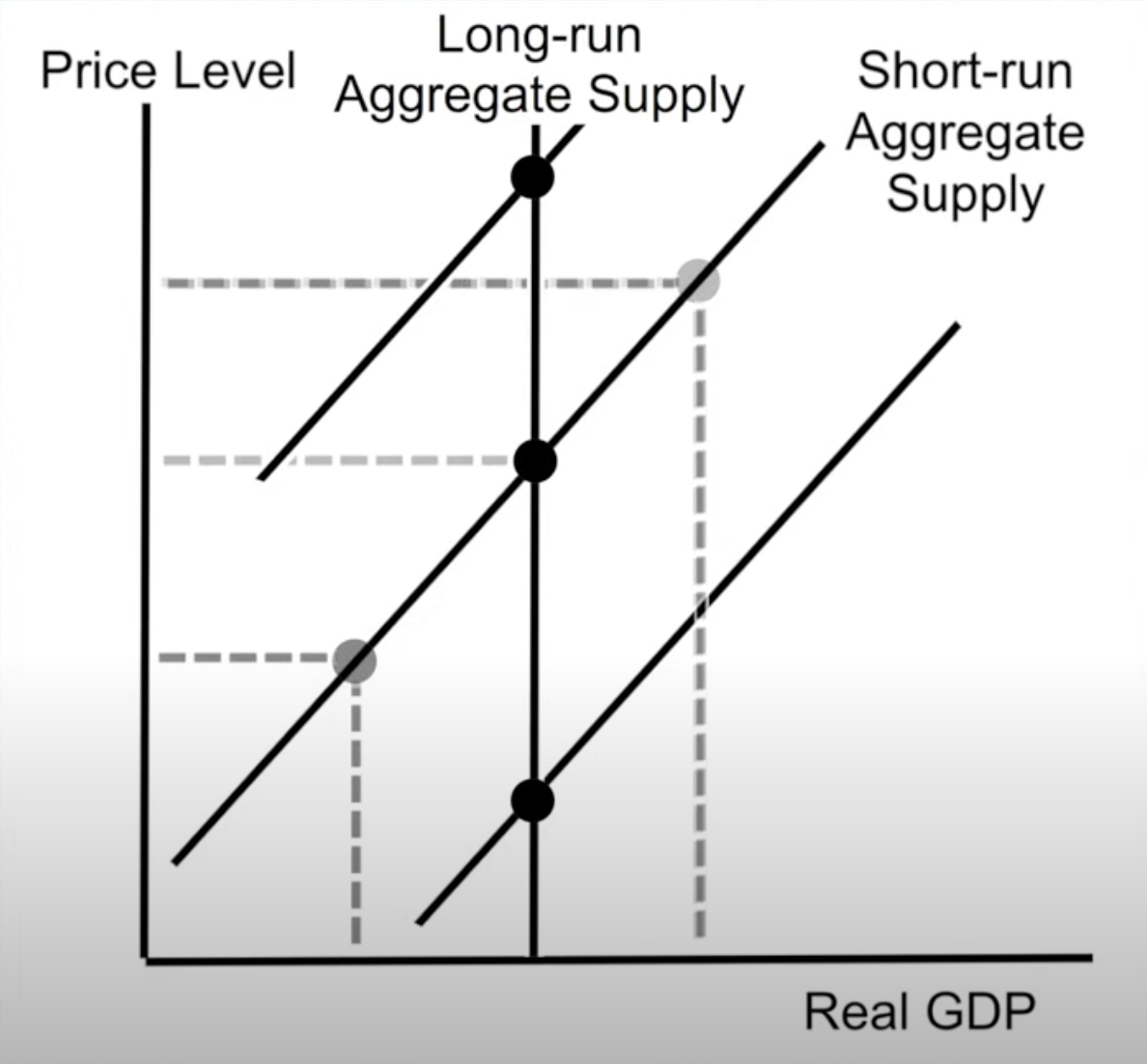
The Long-Run Aggregate Supply Curve is derived from an expected shift in price level within the short-run aggregate supply curve. When the price level is expected to increase, inflation rises, wages rise, and resource costs correspondingly increase. This shifts the short-run aggregate supply curve to the left. Ultimately, this means that the level of output produced when an economy is operating at full employment is what is represented by the long-run aggregate supply.
The primary difference between the short-run aggregate supply curve and the long-run aggregate supply curve are
| SRAS | LRAS | |
|---|---|---|
| Inputs in production | At least one input is fixed | All inputs are variable |
| Slope of curve | Upward-sloping | Vertical at |
| Responsiveness of input prices to changes in the price level | Sticky | Fully flexible |
| Relationship between and | As ↑, ↑ are accompanied by ↓ There is a trade-off | As PL↑, no in and no in There is no trade-off |
Changes in the price level will cause changes in output and employment in the short run, but not the long run.
Essentially:
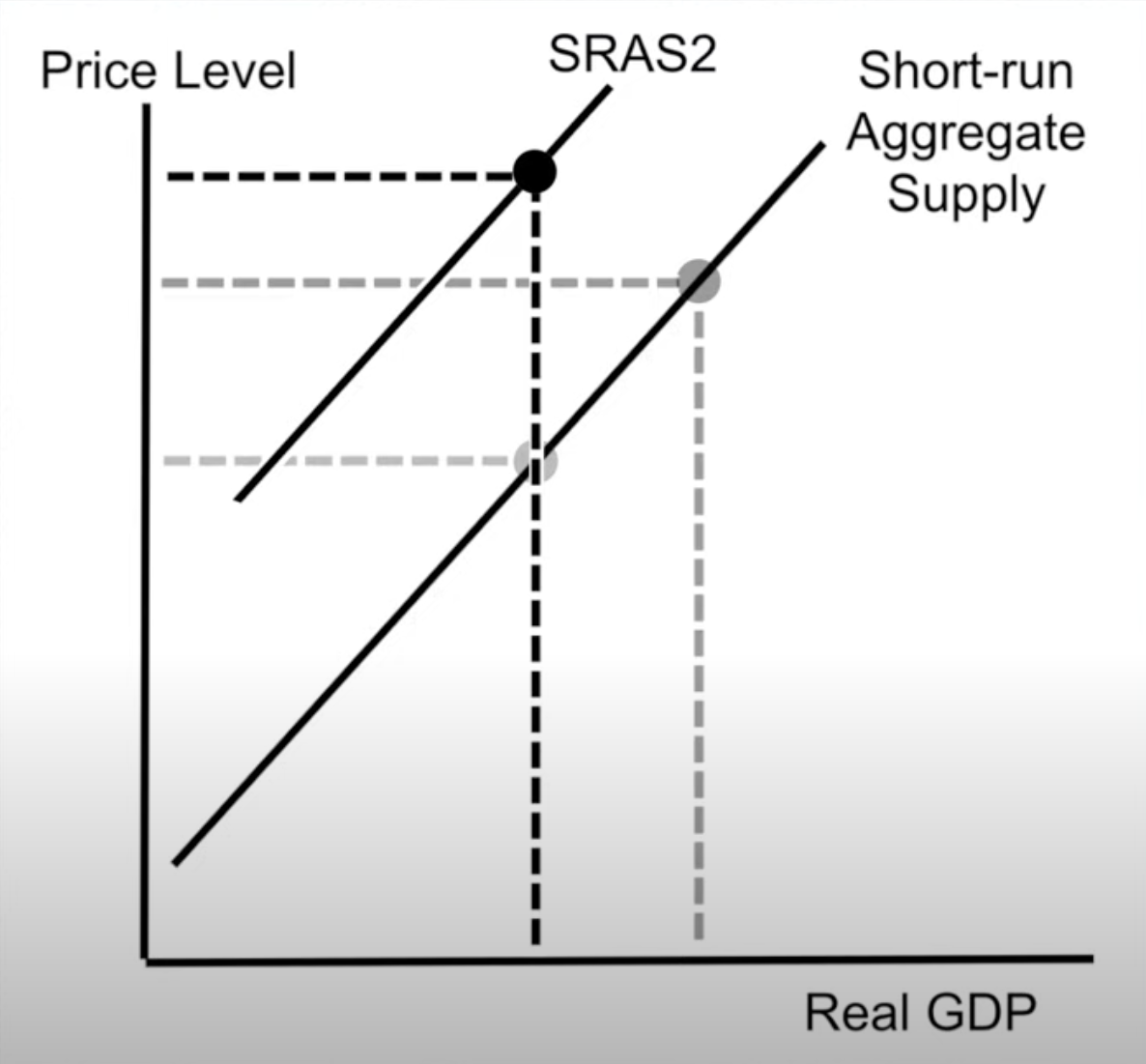
- First, as the price level increases, we move up the supply curve as producers produce more output in the short run
- However, as wages and resources also go up, the short-run supply curve shifts to the left in the long run
Below is an image of the shift in steps one and two:
Similarly, this shift can happen in the opposite direction (where the price level increases). These circumstances describe a new curve: the long-run aggregate supply curve:
This is quite similar to the business cycle and unemployment, and it also represents the same concepts presented in the production possibilities curve. Both curves show our maximum sustaining capacity and the amount we will produce at full employment. Anything that shifts the PPC will also shift the LRAS.
Long Run Aggregate Supply and the Production Possibilities Curve
The PPC describes all combinations of consumer goods and capital goods. Any point on the curve represents full employment (actual unemployment rate = natural unemployment rate). So, a point X on the PPC will represent the quantity of output that the economy is producing at maximum efficiency. This corresponding point on the LRAS represents the value of that output in real GDP.
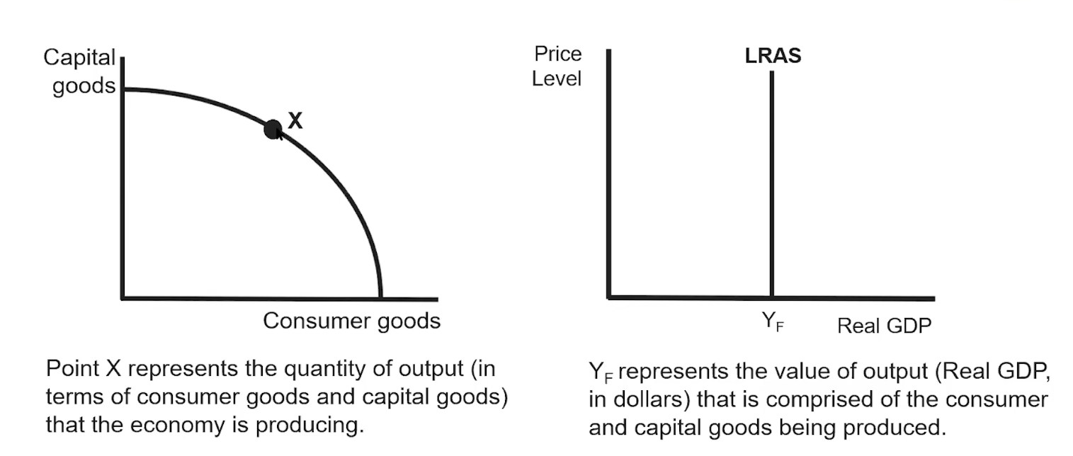
For both the PPC and the LRAS, we refer to the natural rate of unemployment () and not the actual rate of unemployment (). Essentially, a shift in the actual will not shift the PPC or the LRAS, while a shift in the will. Ultimately, the shifters of the Long-Run Aggregate Supply are the same shifters of the PPC, especially a shift in the natural unemployment rate.
Classical vs Keynesian Aggregate Supply
Classical economics is the belief in long-run self-adjustment, and that prices and wages will always counteract output gaps and return back to long-run equilibrium.
The Keynesian model says that the price level doesn’t fall when output is below full employment because wages and resource prices are sticky. Essentially, they claim that price levels don’t shift when aggregate supply shifts; it’s just GDP that shifts. As a result, Keynesian claims that we need outside intervention to fix the economy.
The actual solution is actually a combination of: Keynesian, Intermediate and Classical models.
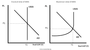
Essentially, as we pass full employment, price level increases as producers compete for limited resources. Conversely, when aggregate demand falls, wages and resource prices are sticky, and we end up with a flat long-run aggregate supply curve.