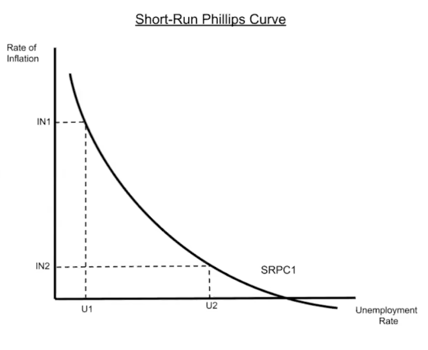
The Phillips Curve shows the relationship between the rate of inflation and the unemployment rate. Essentially, as Aggregate Demand and GDP change, we see the rate of inflation and unemployment (represented by the point on the line) move up and down the graph. Essentially, when inflation is high, unemployment is low. But at the same time, wages are worth less due to a decrease in purchasing power.
Phillips Curve Equilibrium
Similar to the short-run aggregate supply curve and the long-run aggregate supply curve, we have a short-run Philips curve and a long-run Philips curve. The Long-Run Phillips Curve shows the rate of full employment (natural rate of unemployment), and equilibrium occurs when SRPC and LRPC intersect. This essentially means that both our inflationary rate and our unemployment rate is at the equilibrium position where we hope to be in the long run.
Phillips Curve Output Gaps
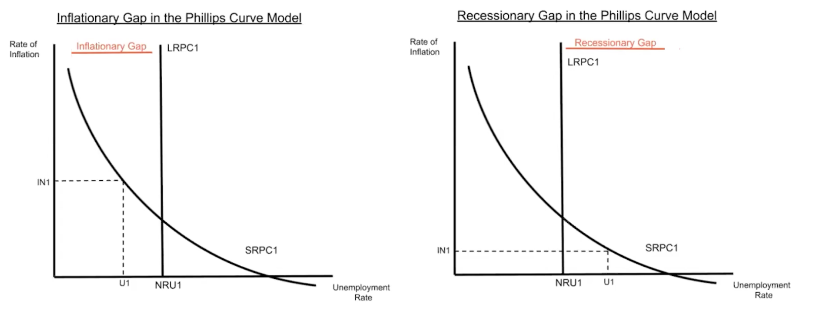
Once again, similar to the aggregate supply curves, we also have inflationary gaps and recessionary gaps. However, in Phillips curves, inflationary gaps are when the short-run equilibrium is to the left of the long-run Phillips curve, and recessionary gaps are when the short-run equilibrium is to the right of the long-run equilibrium position. This is the reverse of what we learned in aggregate supply.
Shifting the Phillips Curve
Demand Shocks
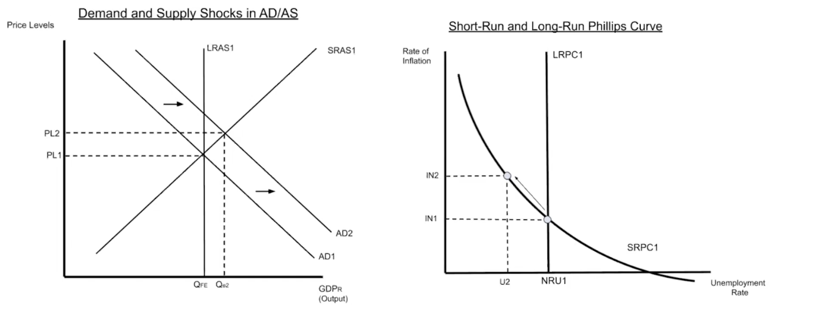
Essentially, all shifts on the aggregate demand curve are in association with a movement along the Phillips Curve. So if aggregate demand shifts to the right, we see the Philips curve point shift to the left. For example, assume that the aggregate demand curve shifts to the right. We know that inflation has now risen. Similarly, since the Phillips curve point will move to the left and up the curve, we can see that the rate of inflation has increased as well. The increase in real GDP on the aggregate demand curve also corresponds with the decrease in the unemployment rate on the Phillips curve.
Supply Shocks
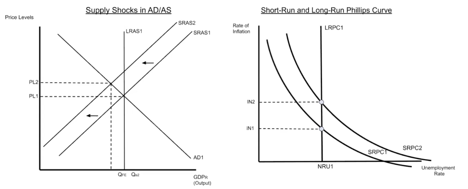
In contrast to demand shocks, all shifts on the aggregate supply curve actually shift the entire Phillips curve (but in the opposite direction). For example, if the aggregate supply curve shifts to the left, we know that there is now an increase in inflation. As a result, the Phillips curve will shift to the right to associate with the change in the rate of inflation.
Long-Run Impacts and Corrections
Once again, similar to [[3.7 — Long-Run Self-Adjustment|]], if a market is not in equilibrium in the short-run, it will eventually shift back to the long-run equilibrium. This is because wages and prices are no longer sticky, which means even if there is inflation, the prices of wages will also increase. Correspondingly, that will increase unemployment and shift the AS curve back to the long-run equilibrium. This has the same effect on the long-run Philips curve.
Shifting the long-run Phillips curve is done by increasing or decreasing structural or frictional unemployment. For example, if the workforce becomes better qualified to fill job openings (structural) or if there is improved job finding time (frictional), the long-run Philips curve will shift to the right.