Reinforcement Learning (RL)

Among Supervised Learning and Unsupervised Learning, Reinforcement Learning is one of the primary neural network learning paradigm, focused on the process of training models in simulation—essentially, rewarding and penalizing an agent in a simulated world to create synthetic data. RL is primarily used in dynamic environments without predefined inputs and outputs. For example, we would use RL to train a model to beat the Snake game by rewarding it for eating apples and penalizing it for running into walls.

On a high level, reinforcement learning primarily consists of an agent and its environment—which is where it lives and interacts. At every step, the agent sees an observation of the state of its environment and then decides on an action to take. Naturally, the environment changes as the agent takes actions within it—and the agent is provided with a reward if its actions helped move the world state towards its intended goal. Intuitively, the agents goal is to maximize its cumulative reward, referred to as its return.

Clearly, reinforcement learning is a very obvious example of biomimicry, in which we’re quite literally classically conditioning (Pavlov’s dog) an agent to achieve a goal we require it to. RL stems from a similar process in animal psychology: biological brains are hardwired to interpret signals such as pain and hunger as negative reinforcements, and interpret pleasure and food intake as positive reinforcements. Animals learn to engage in behaviours that minimize negative reinforcements and optimize the rewards.

When I first heard of the idea of reinforcement learning a little over a year ago, I would this explanation a little too simple and intuitive—but a year later now, even after learning about policy training at K-Scale Labs and reading a handful of landmark papers, RL is still just as intuitive as it first seemed. For the sake of academic accuracy, here is a more accurate description of RL from OpenAI’s Standing Up article:

A state is a complete description of the state of the world. There is no information about the world which is hidden from the state. An observation is a partial description of a state, which may omit information.

In deep RL, we almost always represent states and observations by a real-valued vector, matrix, or higher-order tensor. For instance, a visual observation could be represented by the RGB matrix of its pixel values; the state of a robot might be represented by its joint angles and velocities.

When the agent is able to observe the complete state of the environment, we say that the environment is fully observed. When the agent can only see a partial observation, we say that the environment is partially observed.

The rest of this document is paraphrasing my interpretation of the same article—as well as other papers and resources. (In hindsight, I ended up basically copying the article word-for-word!)

A basic RL agent interacts with its environment in discrete time steps. At each time $t$, the agent receives the current state $S_t$ and reward $R_t$. Then, it chooses an action $A_t$ from the set of available actions. The agent moves to a new state $S_{t+1}$ and new reward $R_{t+1}$. The goal of a RL agent is to learn a policy: $\pi :SxA\to [0,1],\pi (s,a)=Pr(A_t=a|S_t=s)$ that maximizes the expected cumulative reward.**

When the agent’s performance is compared to that of an agent that acts optimally, the difference in performance is described as regret. To act near optimally, the agent must reason about the long-term consequences of its actions (maximize future income), although the immediate associated reward might be negative.

---

Action Spaces

The set of all valid actions in a given environment is often called the action space. Some environments are discrete action spaces, where only a finite number of moves are available to the agent (e.g: chess, Go, Atari). Similarly, some environments are continuous action spaces where actions are represented by real-valued vectors with no finite limit to the action space (e.g: a robot in the physical world).

Policies

A policy, often used synonymously with agent, is the trained network that the agent uses to to decide what actions to take. it can be deterministic or stochastic—but it always serves to maximize cumulative reward.

Depending on the action space, we use different types of stochastic policies: categorical policies for discrete action spaces, and diagonal Gaussian policies for continuous action spaces. Categorial policies are a lot like a classifier model—where we simply build a neural network to classify across the discrete action space.

Reward

The reward function $r_t=R(s_t,a_t,s_{t+1})$ takes in the current state of the world, the action just taken, and the next state of the world; although it is often simplified to just be dependent on the current state $R(s_t)$ or a state-action pair $R(s_t,a_t)$.

Just like Pavlov’s dog, the goal of the agent is to maximize the cumulative reward over an episode. There are two primary ways in which this can be done:

1. Finite-Horizon Undiscounted Return which is simply the sum of rewards obtained in a fixed window of steps: $R(\tau )={\sum }_{t=0}^T{r}_t$
2. Infinite-Horizon Discounted Return which is the sum of ALL rewards ever obtained by the agent—but discounted by how far into the episode they are obtained $R(\tau )={\sum }_{t=0}^{\infty }{\gamma }^t{r}_t$ This discount factor is the same as gamma $\gamma$ which we utilized when training CNNs for ASL fingerspell recognition. Without the discount factor, the total reward in an infinite-horizon setting could be infinite—and $\gamma$ ensures it converges to a finite number by iteratively reducing the size of the rewards. Essentially, this encourages short-term good behaviour and ensures the agent cares more about immediate rewards and than future rewards; because it is highly likely that the agent can’t plan perfectly far into the future.

Value Functions

An important requirement in RL is to be able to assign a value to a state (or a state-action pair); essentially, the expected return if we visit that certain state and act according to a particular policy afterward. There are four primary value functions:

1. On-Policy Value Function which gives the expected return if you start in $s$ and always act according to policy $\pi$
2. On-Policy Action-Value Function which gives the expected return if you start in state $s$, take an arbitrary action $a$ (which may have not come from the policy), and then forever act according to policy $\pi$
3. Optimal Value Function which gives the expected return if you start in state $s$ and always act according to the optimal policy in the environment
4. Optimal Action-Value Function which gives the expected return if you start in state $s$, take an arbitrary action $a$, and then forever act according to the optimal policy in the environment

---

Reinforcement Learning is often represented mathematically via the Markov Decision-Making Process where:

• $S$ is the set of all valid states
• $A$ is the set of all valid actions
• $R:S\times A\times S\to \mathbb{R}$ is the reward function, with $r_t=R(s_t,a_t,s_{t+1})$
• $P:S\times .A\to \mathcal{P}(S)$ is the transition probability function, with $P(s^{\prime }\mid s,a)$ being the probability of transitioning into state $s^{\prime }$ if you start in state $s$ and take action $a$
• and ${\rho }_0$ is the starting state distribution

---

Below is a non-exhaustive diagram representing the taxonomy of algorithms in modern reinforcement learning:

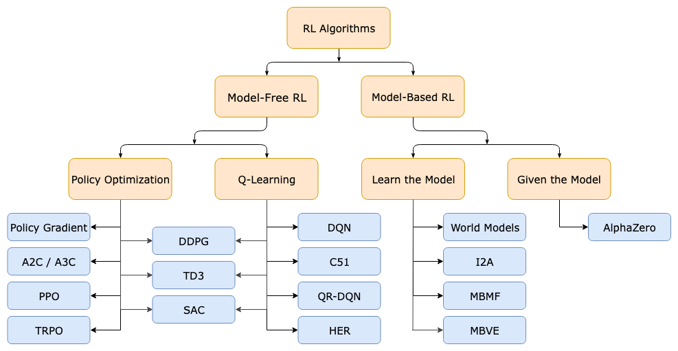
Model-Free vs Model-Based Learning

The primary branching points of RL algorithms (model-free vs. model-based) is whether agents have access to a model of the environment. Essentially, whether the agent can utilize a function that predicts state transitions and rewards.

The primary benefit to model-based RL is that the agent is able to plan by thinking ahead and looking across a range of possible choices; and these results can then learning from planning ahead into a functioning policy. AlphaZero is a famous example of this.

The primary downside is that a ground-truth model of the environment is usually not available to the agent. In this case, if we attempt to use model-based RL, the agent has to discover the environment purely through its own experience—and any error (bias) in this environment can be exploited by the agent. This results in agents that perform well with respect to the learned model, but behave sub-optimally in the real environmentally. From my understanding right now, this seems to be the exact sim2real issue I saw us facing when I just visited K-Scale. Robots are able to walk in simulation (kinda a learned model)—but the same policy doesn’t translate to real life because of so many unexpected variations. “Model-learning is fundamentally hard, so even intense effort—being willing to throw lots of time and compute at it—can fail to pay off.”

What to Learn

Another branching point is what to learn:

• Policies (stochastic/deterministic)
• Action-value functions (Q-functions)
• Value functions
• Environment Models

When dealing with model-free reinforcement learning, there are two main approaches to training:

1. Policy Optimization
   • These algorithms typically represent a policy function very explicitly; and use gradient ascent (Gradient Descent but for maximums instead!) to maximize a score function
   • Usually done on-policy, which means it uses data from its most recent behaviour—rather than older data
   • It often uses a helper value function which estimates how good each state is, and correspondingly guides policy updates
   • Popular policy optimization methods are A3C which performs gradient ascent to directly maximize performance, and PPO which optimizes indirectly via a safer function that doesn’t change policy too wildly
2. Q-Learning
   • These algorithms attempt to learn a function $Q_{\theta }(s,a))$ which attempts to approximate the optimal action-value function $Q^{\ast }(s,a)$. As we saw in earlier value functions, the $Q(s,a)$ function aims to predict the expected future reward if you start in state $s$, take action $a$, and act optimally after that
   • These methods are built on the Bellman equation which essentially states that the value of a state-action pair is the reward you receive now plus the best future value you can get later
   • Q-Learning is often done off-policy, which means it can learn from any data—even if it was collected by a different policy. It balances exploration (trying new things) and exploitation (using the best-known move)
   • The most popular examples of Q-Learning methods are DQNs and C51

The benefit of policy optimization methods is that you directly optimize for what you want, which makes them stable and reliable. In contrast, Q-learning methods indirectly optimize for agent performance by training $Q_{\theta }$ to satisfy a self-consistency equation, which tends to be less stable. At the same time, they are more efficient when they do work, and they can reuse data more effectively. Since policy optimization and Q-learning are not mutually exclusive, there are some algorithms that trade-off between the strengths and weaknesses of both, including DDPG which concurrently learns deterministic policy and a Q-function by using both to improve each other]]