3.5 — Equilibrium in Aggregate Supply and Demand

The Aggregate Supply and Demand Curve is known as the AD-AS model. It includes the ACE framework, which corresponds with the following ACE acronym:

1. Axes
   • Price level, Real GDP
2. Curves
   • Downward Sloping Aggregate Demand Curve
   • Upward Sloping Short-Run Aggregate Supply Curve
3. Equilibrium Points
   • $P{L}_E$ meets $Y_E$

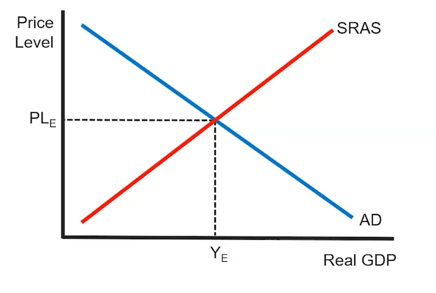
Short-Run Equilibrium

The above ACE acronym and equilibrium is represented in the following graph:

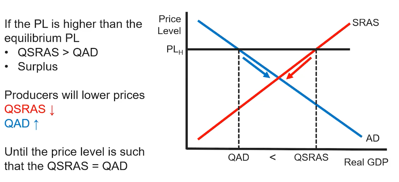
Aggregate Market Disequilibrium

In an instance where the price level is higher than the equilibrium price level, we will essentially have something similar to AP Microeconomics Unit 2.7 Market Disequilibrium. In this case, since the $QSRAS$ is greater than the $QAD$, we will have a surplus. As a result, producers will lower their price which will reduce the quantity $QSRAS$ and correspondingly increase $QAD$ until the price level is such that $QSRAS=QAD$. The reverse will happen if the price level is lower than the equilibrium price level.

This surplus is also similar to 2.6 — Market Equilibrium and Consumer and Producer Surplus.

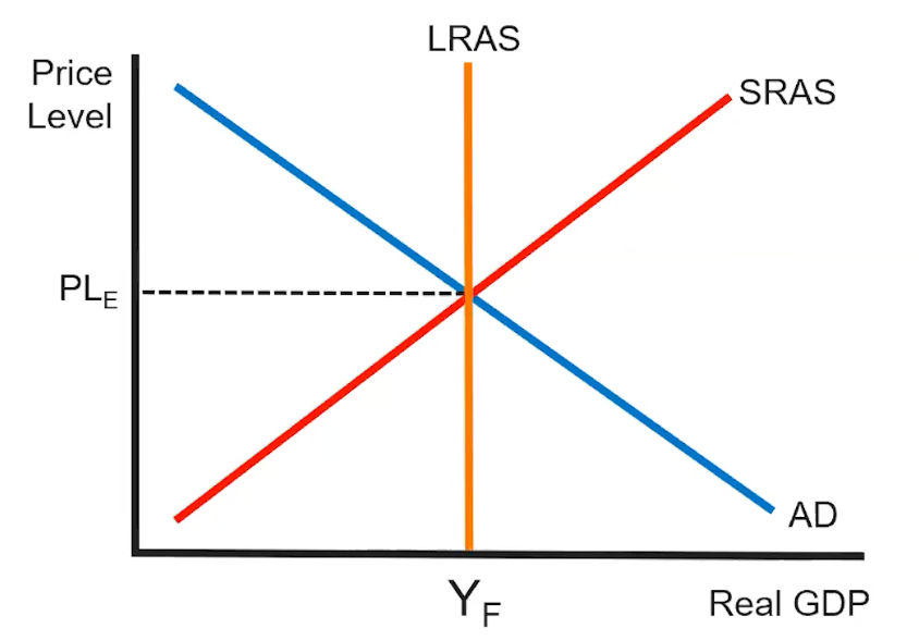
Long Run Equilibrium

When the economy is in long-run equilibrium, the current output will equal the potential output, where the potential output is represented by a vertical $LRAS$ curve at $Y_F$. This is represented through the Long-Run Aggregate Supply Curve.

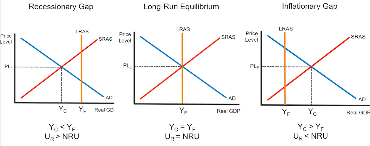
Output Gaps

There can also be disequilibrium in the format of recessionary and inflationary gaps. In an instance where the long-run equilibrium quantity is greater than the short-run equilibrium quantity, we have a recessionary gap. Similarly, in an instance where the long-run equilibrium quantity is less than the short-run equilibrium quantity, we have an inflationary gap. This is represented in the following graphs: