In the long run, all inputs are variable, and firms can adjust their scale of production. This flexibility allows firms to minimize costs by choosing the most efficient input combination for a given level of output.
Economies and Diseconomies of Scale
As firms increase production, their costs per unit may decrease, remain constant, or increase:
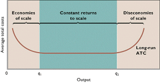
- Economies of Scale: Long-run average total cost () decreases as output increases. This occurs due to factors like specialization, bulk purchasing, and improved technology.
- Constant Returns to Scale: remains constant as output increases. This happens when a proportional increase in all inputs leads to the same proportional increase in output.
- Diseconomies of Scale: increases as output increases. This results from inefficiencies like communication breakdowns or coordination challenges in large firms.
In simpler terms, there are three possible outcomes, given in the following example: Assume a firm is producing 100 bikes with a fixed number of resources (workers). If the firm decides to double the resources, what happens to the number of bikes?
There are three possibilities:
- It will double (constant return to scale)
- Both resource and output increase equally
- It will more than double (increasing returns to scale)
- Output increase is greater than resource output
- It will less than double (decreasing returns to scale)
- Output increase is less than resource output
Long-Run Average Total Cost (LRATC) Curve
The curve is derived from a series of short-run ATC curves, each representing a specific plant size or scale of production. The is U-shaped because:
- Initially, economies of scale reduce costs as production expands.
- Eventually, due to the Law of Diminishing Marginal Returns, diseconomies of scale increase costs as production grows too large.