But how do AI images & videos actually work? — Welch Labs

Video

CLIP

• In February 2021, a team at OpenAI released a new model architecture called Contrastive Language-Image Pretraining (CLIP)
  • It is composed of two models: one processes text, and the other images
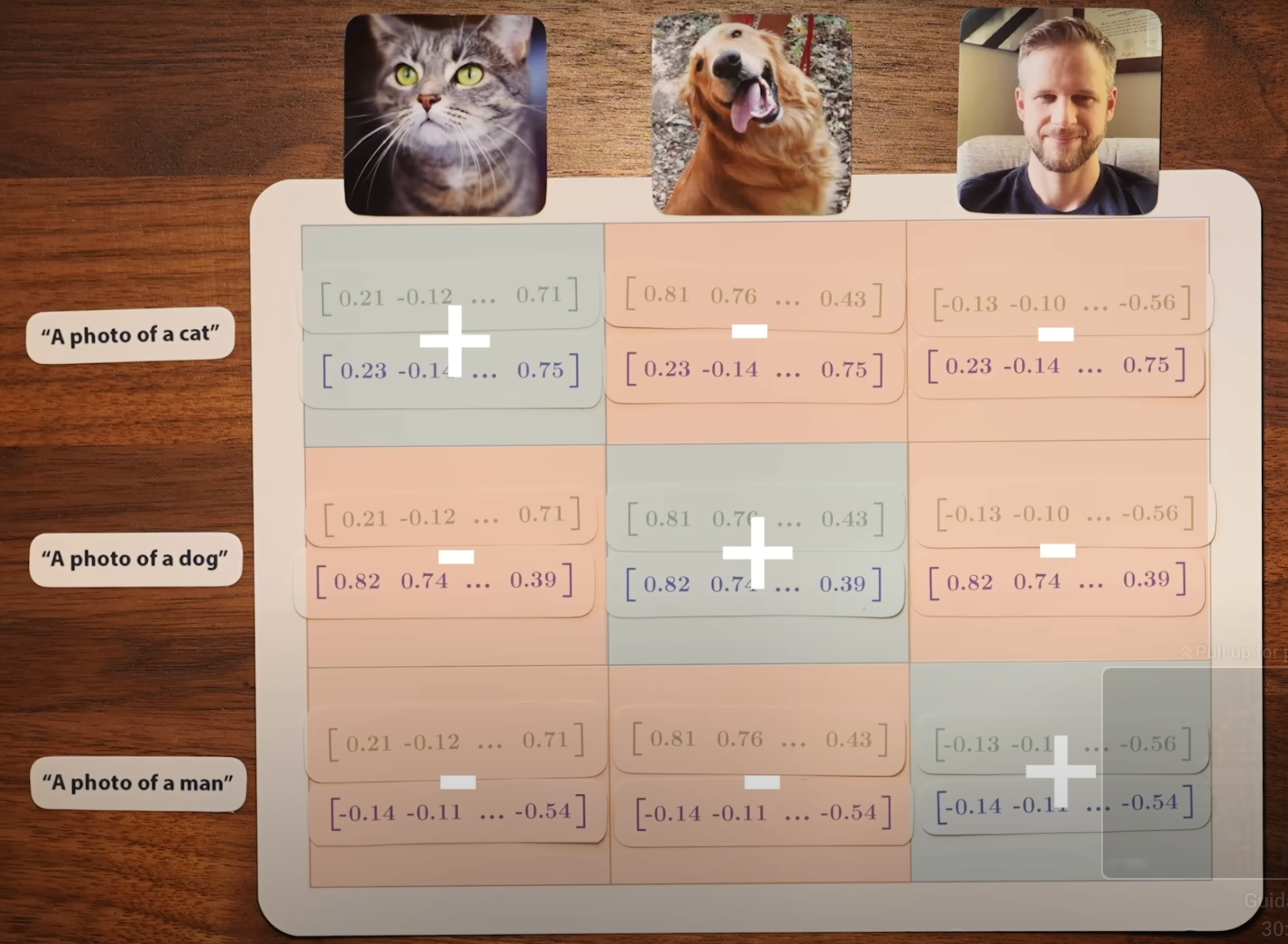
  • The central idea is that the text encoder and image encoder have similar vectors for an image and its associated caption
• To achieve this, they used Contrastive Loss; essentially, the CLIP training objective is to maximize the similarity between matching image-caption-pairs, while minimizing the similarity of mismatched pairs:
  • Since they measure similarity via Cosine Similarity, the image and text models in CLIP are trained to maximize the alignment between related image-text pairs, while minimizing the angular alignment between unrelated pairs
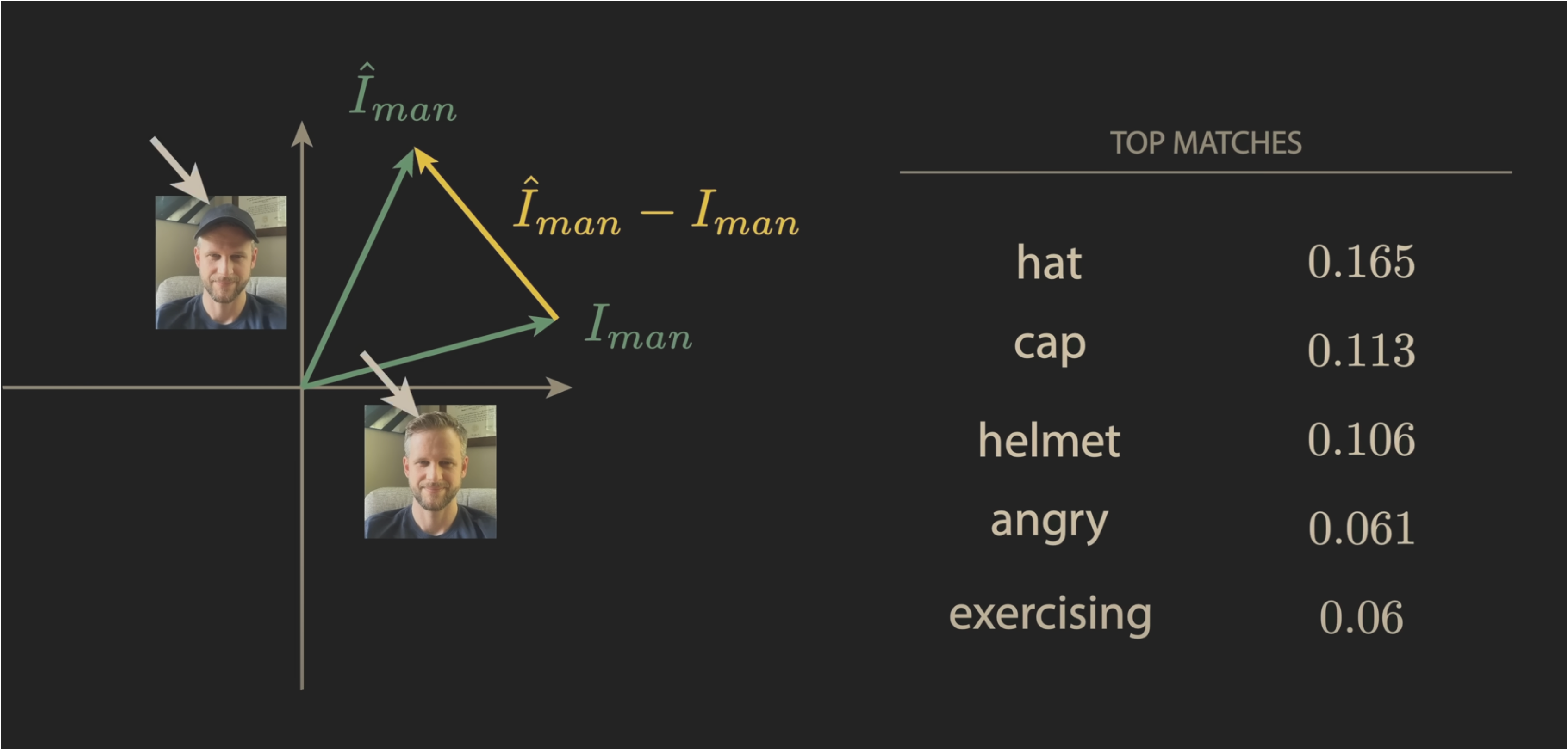
• Just like most embedding spaces, this latent space has many interesting properties. For example, when subtracting the vector representations of two images (one of a man with a hat, and one without), the closest matching text embedding for the difference vector are of the words “hat” and “cap”:
• However, while the CLIP model can map image and text to a shared embedding space, we have no way of generating images/text from our embedding vectord

Diffusion

• With 2020’s breakthroughs in language modelling, a team at Berkeley came out with a paper titled Denoising Diffusion Probabilistic Models (DDPM), showing that it was possible to generate high-quality images with a diffusion process
  • Essentially, we take a set of training images and add noise step-by-step, until the image is destroyed
  • Then, we train a neural network to iteratively reverse this process
• However, unlike the common perception that diffusion simply reverses the noising process one step at a time, Diffusion models actually operate differently:
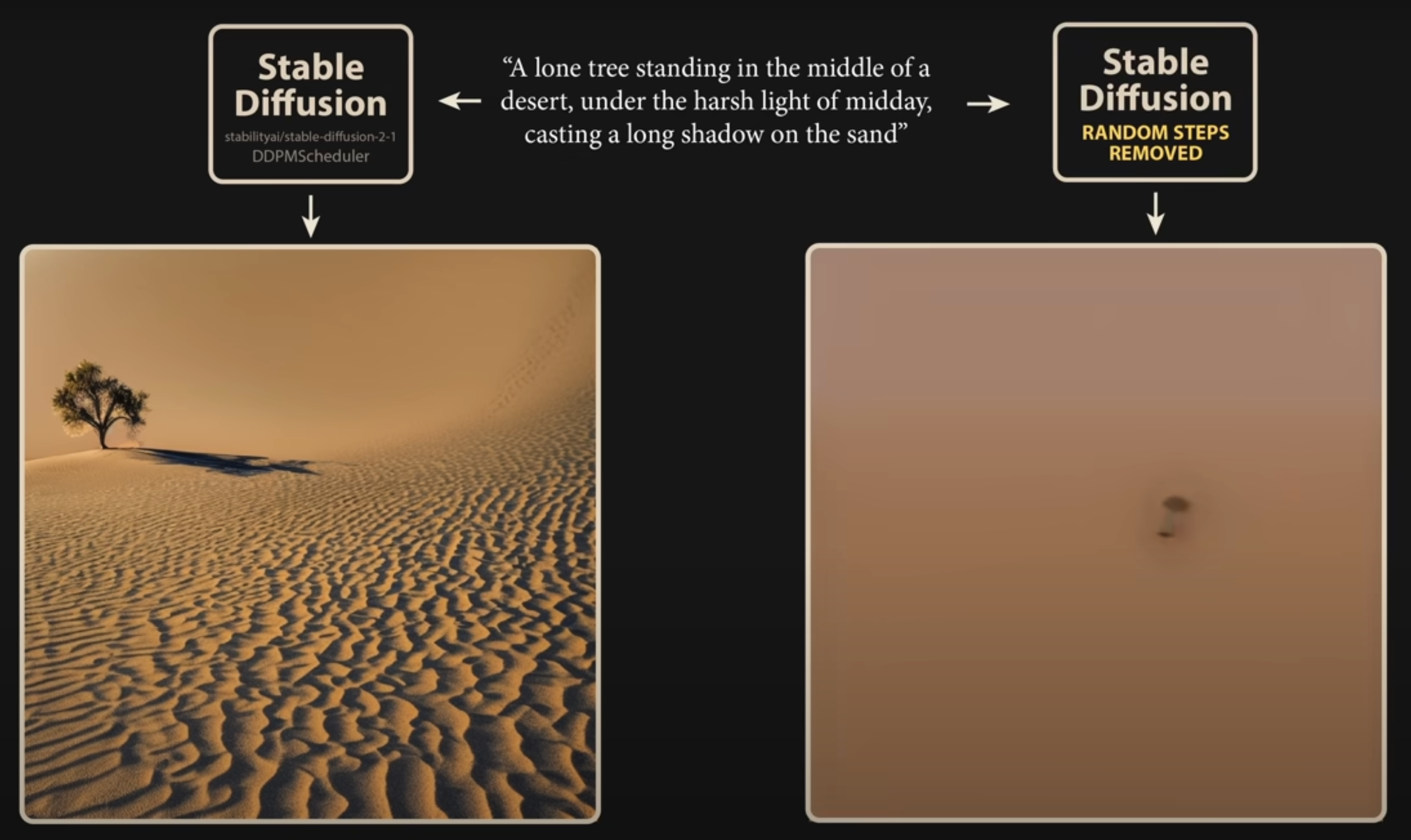
  • Interestingly, instead of only adding random noise during the training process, we also add random noise to images during image generation (after each step where we predict a less noisy image) before passing it back to the model.
    • Here on the left is an image with random noise added during each step of the image generation process, and on the right is an image generated without:
  • Additionally, in contrast to training models to reverse a single step in the noise-addition process, we take an initial clean image $x_0$ and add scaled random noise $ϵ$; then, they train the model to predict the total noise that was added to $x_0$
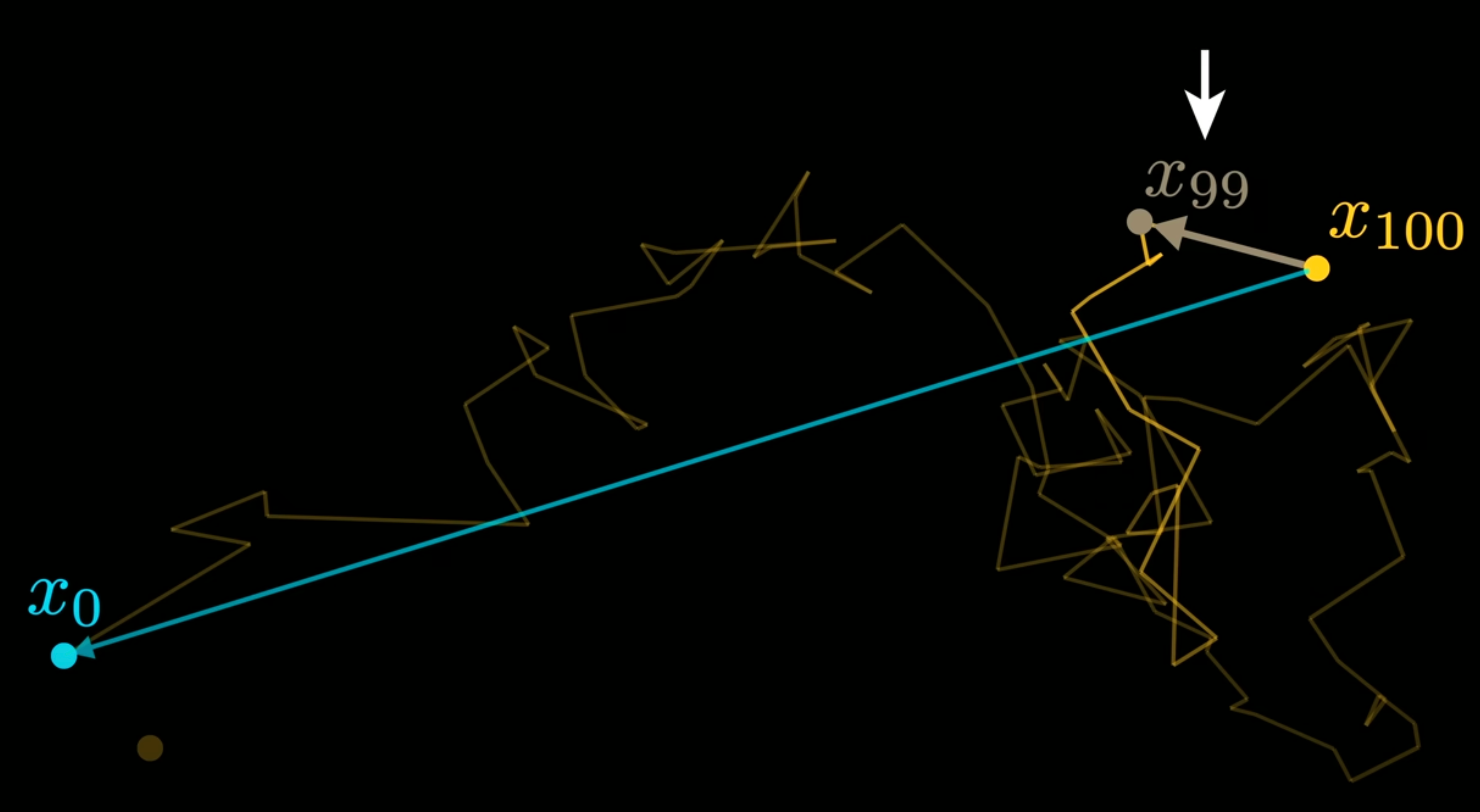
    • One way to visualize this is through the following image:
    • Assume that, in the above image, the $x_0$ is the initial position of a vector in our latent representation of the image, and we take a 100 random noise-adding steps that randomly change the position of this vector. It is more straightforward to predict the total noise added across the entire noise-adding process (distance from $x_{100}$ to $x_0$) instead of predicting each of the 100 individual random de-noising steps

Prompt Guidance